From Transformers to ChatGPT
This note provides a high-level summary of the progress in large language models (LLMs) covering major milestones from Transformers to ChatGPT. The note serves as a fast-paced recap for readers to catch up on this field quickly.

Introduction
Large language models such as GPT-3 have shown impressive performance not only in NLP benchmarking tasks but also blew the public's minds through application interfaces such as ChatGPT.
This note provides a high-level summary of the progress in large language models (LLMs) from 2017 (the inception of the Transformer model) to now (the end of 2022), serving as a fast-paced recap for readers to catch up on this field quickly. General familiarity with machine learning/deep learning is assumed.
This note will only cover a small, core set of papers: Transformer, BERT, GPT, GPT-2, GPT-3, and InstructGPT. There are undoubtedly many other notable papers published during the same period of time - I'll leave them to a literature survey/reading list.
This is a somewhat long note - it is broken down into the following sections: (Please use the Table of Content on the right to navigate)
- Overview
- What is NLP
- Past progress (pre-2017)
- Recent progress (2017 - 2022)
- Model details
- Transformer
- GPT
- BERT
- GPT-2
- GPT-3
- From GPT-3 to ChatGPT
- Conclusions & Reflection
1. Overview
1.1 What is NLP?
Natural Language Processing (NLP) involves a wide range of tasks that focus on the processing and understanding of human language. Some of the main tasks in NLP include Text Classification, Named Entity Recognition (NER), Sentiment Analysis, Machine Translation, Information Retrieval, Question Answering, and Text Summarization. A more complete list of typical NLP tasks and progress in each is available here.
Here are a few excellent references:
- Linguistic basics: Emily Bender’s Linguistic Fundamentals for Natural Language Processing: 100 Essentials from Morphology and Syntax (2013)
- Yoav Goldberg’s book Neural Network Methods for Natural Language Processing (2017)
- Chris Manning’s lectures (CS224d) on Natural Language Processing with Deep Learning (Youtube)
1.2 Past progress (pre-2017)
Historically Natural Language Processing (NLP) was primarily based on rule-based approaches or statistical models. Deep learning took over NLP in the mid-2010s, with Recurrent Neural Networks (RNNs) and Long Short-Term Memory networks (LSTMs) being the de-facto models (there are some minor attempts in other types of models but nothing super successful yet).
The field has made a big jump due to the introduction of these models, but at the same time felt a bit stagnant/limited especially compared to Computer Vision (CV). Let's maybe make a comparison between the status of CV and NLP in the table below.
| NLP | CV | |
|---|---|---|
| Model Scaling | Poor | Good |
| Dataset Size | Small | Large |
| Model Transferability | Poor | Good |
RNN/LSTM are autoregressive models, and because of that, the training is fundamentally sequential and harder to parallelize (e.g., a piece of text reading from left to right). Model scaling in NLP has been behind CV - where model architecture such as Convolutional Neural Networks (CNN) offers much easier parallelization.
Another difficulty scaling in NLP is the lack of large, labeled data set. In CV, we have datasets like ImageNet, with ~1M images tagged with 1000 categories. Although we could potentially construct datasets with ~1M pairs of sentences in machine translation, the information (and model supervision) we could generate from sentence pairs is probably 1 to 2 orders of magnitude lower than an image.
On model transferability, in NLP, we haven't seen the kind of success we saw in CV, where a pre-trained model (on a supervised learning dataset) achieves strong performance on downstream tasks. This is partly due to the diversity of NLP tasks, but equally important is the lack of large labeled datasets to train a good and large enough model that transfers and generalizes well.
One side effect is that we see a significant gap in generation capabilities in NLP vs. CV. Photorealistic images and video generation (e.g., DeepFake) have been around for several years (based on VAE, GAN, etc.), while text generation capability has been extremely primitive- which is also why the recent capability in ChatGPT is seemingly unbelievable.
1.3 Recent progress (2017 - 2022)
The progress from 2017 to 2022 changed all of the above constraints in NLP and made it leapfrog CV. This period of time is indeed the breakthrough period for NLP. We'll talk through the details in the sections below. Here is a preview of the significant changes.
Transformer
Although initially developed specifically for machine translation, Transfomer quickly became NLP's new standard model architecture, largely replacing RNNs and LSTMs. The model architecture allows modeling sequences without having to be autoregressive. This massively improved our ability to scale up the model. More recently, Transformer has gone beyond NLP and has been used to model images and videos and in multi-modal applications, and it is considered to be one of the most important core model architectures in machine learning generally.
BERT, GPT
Thanks to the foundation laid out by the Transformer model, BERT and the GPT-series models could scale up the model size from 100M (GPT and BERT-base) to 175B parameters (GPT-3) in a short span of 2 years. Researchers also found creative ways to leverage large unlabelled datasets to support model size scaling.
A key innovation from GPT and BERT is the clever structuring of pre-trained language model input/output to allow the pre-trained models to be transferred (fine-tuned) for a wide array of NLP tasks. Thus, we established a familiar pre-training + fine-tuning setup we saw in CV, with compelling model performance and transferability.
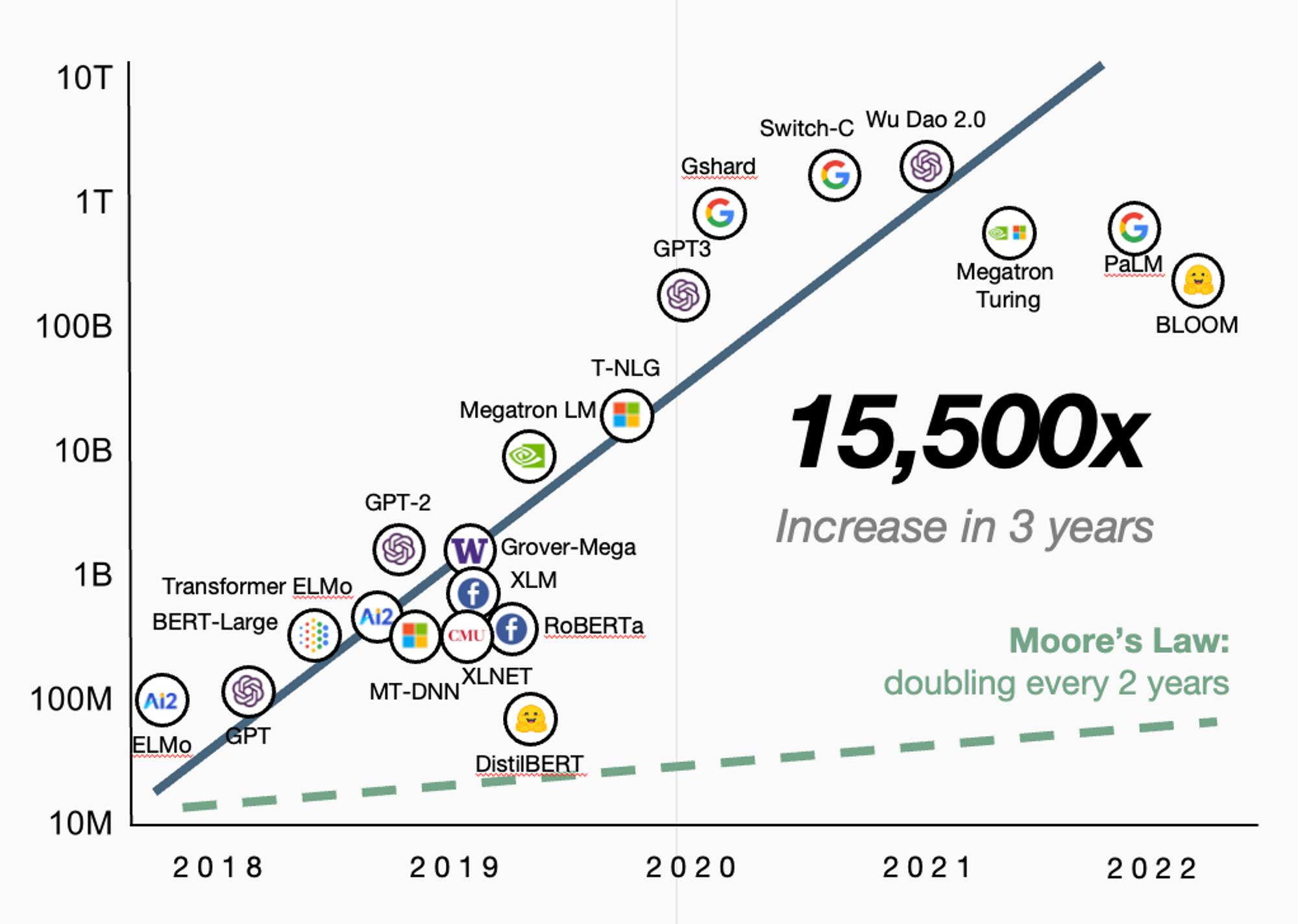
GPT-2, GPT-3
In GPT-2 and GPT-3, the authors introduced the new paradigm of not further adjusting the model (i.e., fine-tuning), but instead of they use natural language "prompts" to tell the model to perform new tasks. The prompts can potentially include some examples (aka, demonstrations). This is called a zero-shot or few-shot setting (depending on how many examples are given to the model).
This allows much-improved transferability since we no longer need to collect a labeled dataset for each specific downstream task, i.e. the model works out of the box on new tasks without any further fine-tuning! This is a significant new step towards making a pre-trained model capable of performing previously unseen tasks completely based on the context/prompt user provides and engaging in open-ended tasks such as doing classifications on an unknown set of labels, engaging in dialogs, writing code, etc. - activity starts to resemble reasoning and intelligence.
From GPT-3 to ChatGPT
Fundamentally, GPT-3 is just a language model. When given a piece of text (i.e., prompt), it generates, somewhat randomly, plausible subsequent text that fits the best. This objective is misaligned with “following the user’s instructions helpfully and safely.” InstructGPT focuses on effectively aligning large language models such as GPT-3 with user intent through fine-tuning with human feedback so that the output can be more helpful, truthful, and harmless.
2. Models
2.1 Transformer
Attention Is All You Need (6/2017)
Transformer has an encoder-decoder architecture, as illustrated below. It was originally designed for Neural Machine Translation (NMT) applications. On the encoder side, the Inputs are the sequence of tokens (e.g., words, BPE tokens, WordPieces, etc.) represented by their embeddings. The model sees the input sequence at once.
On the decoder side, the model would start with an empty sequence and output the probability of the next token (at the top of the diagram, labeled as "Output Probability"), then append this token to the output sequence, and use that as the input (at the bottom of the diagram) then predict the next token and repeat this procedure.
During training time, this can be parallelized, because of available ground truth sequence. But at inference time, the decoding can't, in principle, be parallelized (future optimization).
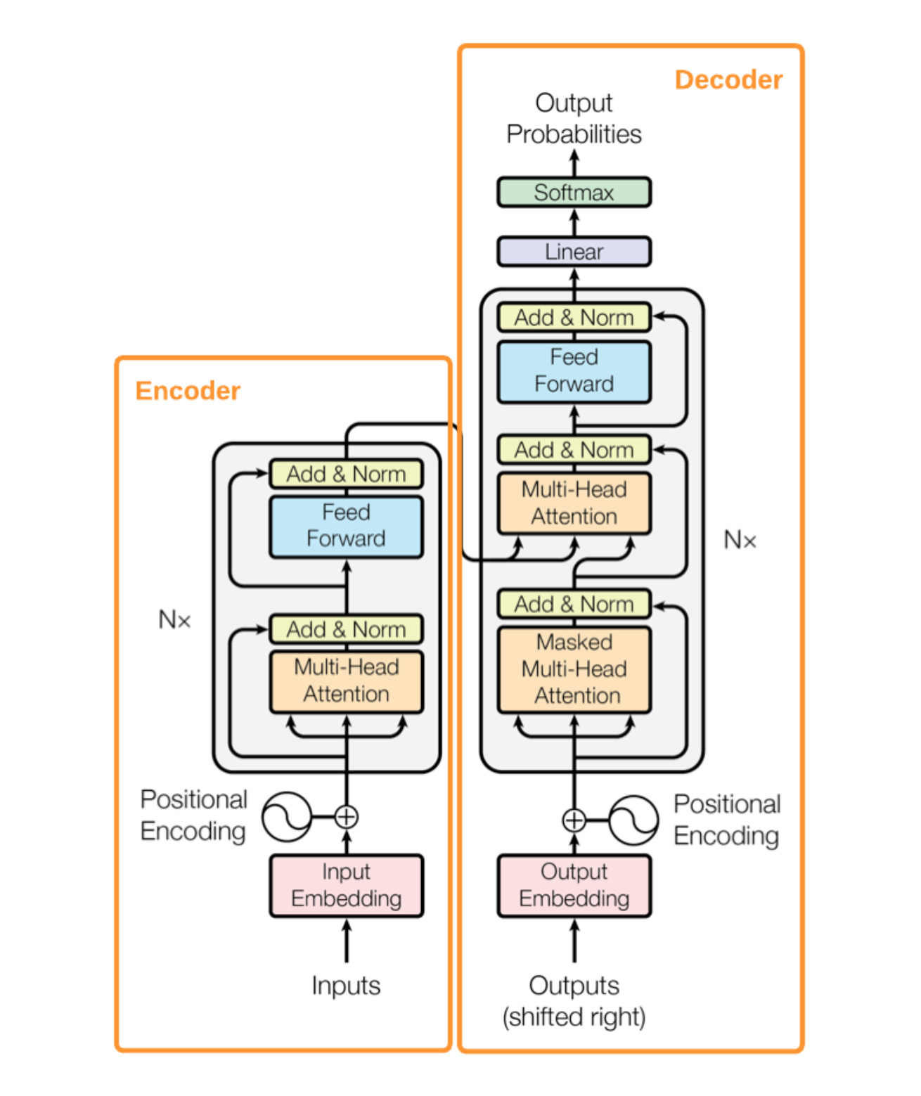
There are many blog posts explaining Transformer in detail when it first came out, e.g., The Annotated Transformer. So here, I'll stay at a pretty high level and focus on the highlights.
The main innovations are really two things, in my opinion:
- Multi-Head Attention
- Positional Encoding
2.1.1 Attention and Multi-Head Attention
The model takes a sequence of tokens (specifically, their embeddings) as the input. What the Attention mechanism does is put each token into its "context". The Attention operation would output an adjusted embedding for each token that takes account of its surrounding tokens while putting emphasis on the ones that matter semantically (i.e., pay attention to them).
For example, in the figure below, in the sentence on the left, “it” refers to the animal, and in the sentence on the right, "it" refers to the street. The Attention mechanism allows the model to correctly associate "it" with what it refers to.
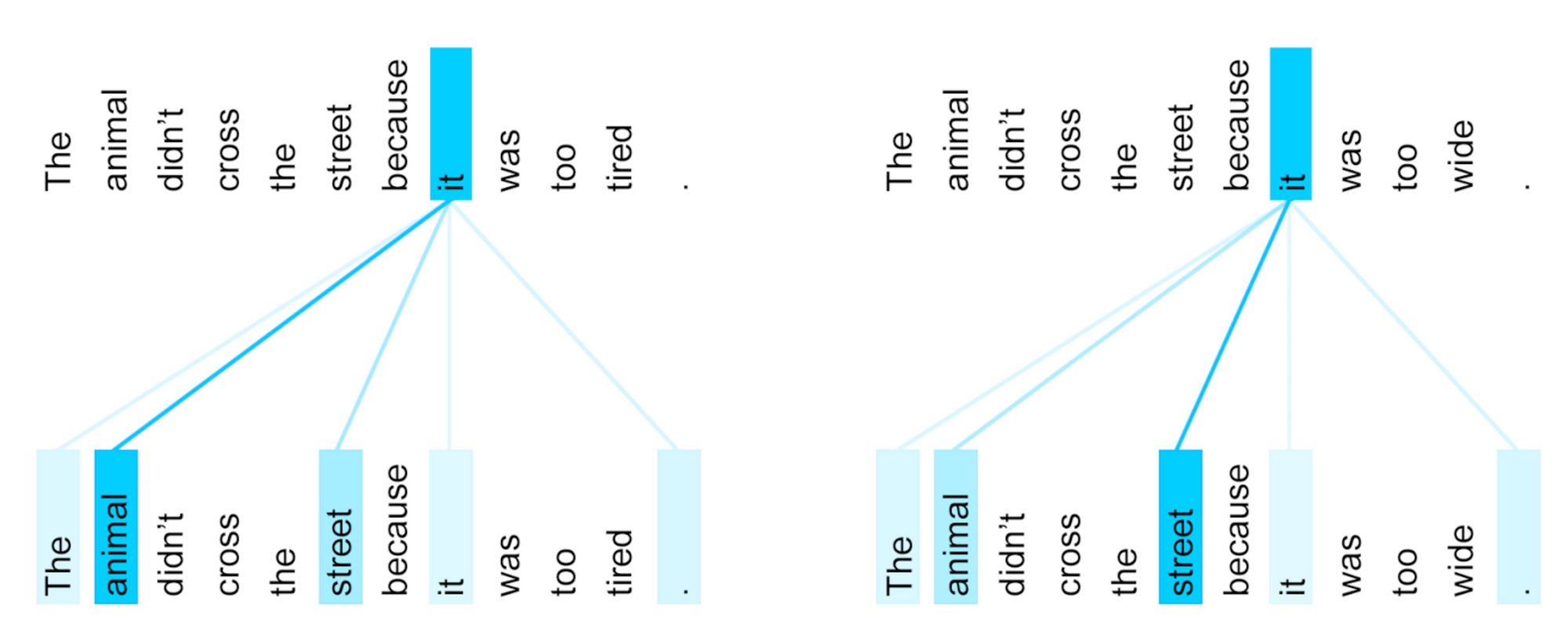
Next, let's see how Attention is implemented.
Attention involves matrices queries (Q), keys (K), and values (V); each can be considered a sequence of vectors. Basically, a query $q_i$ and a list of keys $k_j$ would compute a list of affinity (similarity) factors $a_{ij}$, which then function as the weighting factors to compute a weighted sum of a list of values $v_j$, so the result $r_i=\sum_{j}{a_{ij} v_j}$. In matrix form, it is thus defined as follows:
$$ \mathrm{Attention}(Q, K, V) = \mathrm{softmax}(\frac{QK^T}{\sqrt{d_k}})V $$where $d_k$ is the dimension of the queries and keys vectors and $d_v$ is the dimension of the value vectors.
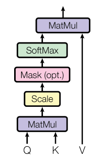
The division by $\sqrt{d_k}$ inside the softmax function is to make the output distribution more "flat" (a.k.a to increase the "temperature" of the softmax). This helps the model find more gradient during training, and the particular choice of $\sqrt{d_k}$ as a normalization factor here is due to the fact that for two random vectors of size $d_k$ with mean 0 and variance 1, their dot product would have mean 0 and variance of $d_k$.
When Q, K, and V are the same sequence (e.g., in the encoder), it is called self-attention. What the attention mechanism does is allow the output embedding (at each position of the output) to be a differently weighted sum version of the input sequence embedding, thus modeling the dependencies of one token on all the other tokens in the sequence, and, notably, this is done without additional hops (all in one matrix operation).
When part of V is masked for reasons during training to not see future ground truth tokens before making a prediction, it is called masked attention (e.g., near the input of the decoder).
In the decoder, there is “encoder-decoder attention”, where queries (Q) come from the previous decoder layer, and the memory keys (K) and values (V) come from the output of the encoder. This allows every position in the decoder to attend over all positions in the input sequence.
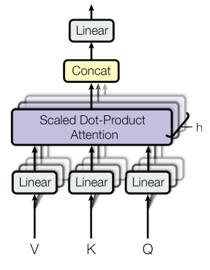
Multi-Head Attention is a small extension where we use learned matrices $W_i^Q, W_i^K \in \mathbb{R}^{d_{model} \times d_{k}}$, and $W_i^V \in \mathbb{R}^{d_{model} \times d_{v}}$ to project $Q, K, V \in \mathbb{R}^{n_{seq} \times d_{model}}$, first before applying the original attention formula. We would have $h$ versions of such matrices, namely $h$ heads. Each output matrix $head_i \in \mathbb{R}^{n_{seq} \times d_{v}}$ will be concatenated and then projected by $W^O \in \mathbb{R}^{hd_{v} \times d_{model}}$. Multi-head attention allows the model to jointly attend to information from different representation subspaces at different positions. With a single attention head, averaging inhibits this.
$$ \begin{split} \mathrm{MultiHead}(Q, K, V) &= \mathrm{Concat}(head_1, ..., head_h)W^O\\\\ \mathrm{where}\enspace head_i &= \mathrm{Attention}(QW_i^Q, KW_i^K, VW_i^V) \end{split} $$where $W_i^Q \in \mathbb{R}^{d_{model} \times d_{k}}$, $W_i^K \in \mathbb{R}^{d_{model} \times d_{k}}$, $W_i^V \in \mathbb{R}^{d_{model} \times d_{v}}$, and $W^O \in \mathbb{R}^{hd_{v} \times d_{model}}$.
2.1.2 Positional Encoding
With Attention, we are able to model the cross dependencies of tokens at different positions of a sequence. However, the attention mechanism is permutation invariant, i.e., it would produce the same results if you scrambled the ordering of the tokens in the sequence. So it is important to encode the order of information.
The paper proposed sinusoidal positional encoding, though later work also used learned encoding with a somewhat similar performance. The eventual input to the model is a sum of the position embedding and the token embedding.
2.1.3 Point-wise Feed Foward Networks
This is the "Feed Forward" block in the diagram. It is basically a multi-layer perceptron (MLP) with ReLU activation. The reason it is called point-wise is that the same MLP is applied to each token in the sequence. In the following equation, $x$ represents the embedding of one token, e.g., length of $d_{model}=512$.
$$\mathrm{FFN}(x) = \mathrm{max}(0, xW_1+b_1)W_2+b_2$$
where $W_1 \in \mathbb{R}^{d_{model} \times d_{ff}}$, $W_2 \in \mathbb{R}^{d_{ff} \times d_{model}}$, $d_{ff}$ is the hidden layer size (e.g., 1024), and $d_{model}$ is the input and output size which is also the embedding size (e.g., 512).
2.1.4 Residual Connection and LayerNorm
This is the "Add & Norm" block in the diagram. Here we are connecting the input and the output of a layer, sum them together, then apply normalization:
$$\mathrm{LayerNorm(x + \mathrm{Sublayer}(x))}$$
LayerNorm is different from the more commonly used (especially in CV) BatchNorm. BatchNorm applies standardization (mean=0, variance=1 after normalization) on each feature across a batch during training. During inference, a global mean and variance are stored and used. LayerNorm applies standardization on each sample across all features. Since this operation is per sample, no global stats are needed. LayerNorm is more commonly used in models of variable length sequences where between-sample variance could be significant/noisy.
2.1.5 Results and Conclusions
The paper mainly focused on machine translation-related experiments, which showed state-of-the-art performance at the time. The particular results are less relevant, so here we focus on general conclusions.
The following table shows a comparison of the complexity scaling (focus on the first two rows), showing that compared to recurrent networks, the transformer avoided long path length and sequential operations, but its overall computation complexity per layer is very similar to recurrent networks.

By the way, "Attention is all you need" is a bit of a misnomer. In follow-up studies, the residual connection, layer normalization, point-wise feed-forward layer, and positional embedding are also critically important for the model's performance. [TODO: add reference]
2.1.6 Hyperparameters and Model Size
Here is the list of hyperparameters for the model:
- $L$: number of repeating transformer blocks/layers.
- $d_{model}$: the embedding size of the input tokens (due to the residual connections, all embedding sizes are the same throughout the model).
- $d_{ff}$: feed-forward hidden layer size. Sometimes, it scales with $d_{model}$, e.g., $4\times d_{model}$.
- $h$: number of heads in Multi-Head attention.
- $d_k$: the dimension of each key and query vector and $d_v$: the dimension of each value vector. Typically, $d_v=d_k=d_{model}/h$.
- $n_{vocab}$: number of tokens in the vocabulary.
- $P_{drop}$: dropout rate
With this above, we can calculate the model parameter as follows:
$$ \begin{split} n_{ff} &= 2 \times d_{model} \times d_{ff} + d_{ff} + d_{model} \approx 2 \times d_{model} \times d_{ff} \\\\ n_{attention} &= 4 \times d_{model} \times d_{k} \times h = 4 \times d_{model}^2\\\\ n_{encoder} &= L \times (n_{ff} + n_{attention})\\\\ n_{decoder} &= L \times (n_{ff} + 2*n_{attention})\\\\ n_{embeddng} &= n_{vocab} \times d_{model}\\\\ n_{total} &= n_{embeddng} + n_{encoder} + n_{decoder} \end{split} $$We can see that model size scales linearly with the number of layers $L$ and quadratically with embedding dimensionality $d_{model}$.
If we use the hyperparameters of the "base" model in the paper: $L=6$, $d_{model}=512$, $d_{ff}=2048$, $h=8$, $d_k=d_v=d_{model}/h=64$ and $n_{vocab}=37000$, we get $n_{total} \approx 19\mathrm{M} + 19\mathrm{M} +25\mathrm{M} = 63\mathrm{M}$ parameters.
2.1.7 Data Efficiency vs. Performance Ceiling
It is interesting to note that, in later work, people found that Transformer is actually quite data-hungry. Part of this is likely because it made fewer assumptions on the structure of the data (either text sequence or image pixel layout). This lack of assumption both made training less data-efficient but also possibly allowed the model a higher performance ceiling which gave rise to the phenomenal we saw that model performance kept improving as we increased the model size in a log-linear fashion (i.e., exponential model size increase in exchange for linear performance improvement), and this trend isn't saturating yet.
2.1.8 Encoder vs. Decoder
Later models sometimes use only the Encoder or the Decoder part of the original transformer model. A few notes about the differences between the encoder and decoder:
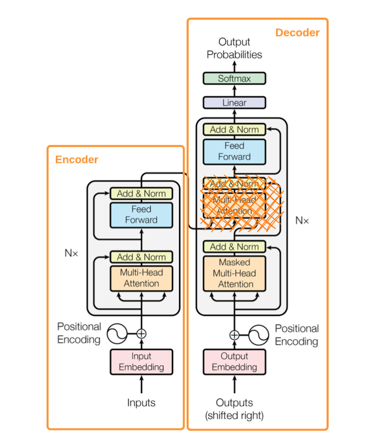
- The encoder outputs a sequence of embeddings corresponding to the sequence of input tokens, while the decoder output a single embedding corresponding to the next token before feeding that into a final linear layer and softmax layer to convert to probability.
- Because of the above, the decoder seems more natural for fine-tuning downstream tasks (as we will see, GPT uses this setup), or for text generation use cases (e.g., ChatGPT). But we also will see BERT used an encoder setup with special tokens designated for use for downstream predictions.
- Additionally, because the decoder is set up to predict the next token(s), its input is configured with a masked attention unit to avoid looking ahead of future tokens in the sequence during training.
- Finally, when we use the decoder alone, we can remove the cross-attention between the encoder and decoder (the crossed-out part in the following illustration). After that, the encoder and decoder block basically look the same except for the masked attention part and the output structure (as discussed in point 1).
2.2 GPT
Improving Language Understanding by Generative Pre-Training (6/2018)
Overview
The main thesis of this paper is that, given that we don't have lots of labeled data for NLP for pre-training, we can rely on unsupervised training on unlabeled text corpus data. This is called generative pre-training because the training objective is language modeling, i.e., predict/generate the next token. After that, we can adjust the pre-trained model to work on downstream tasks with smaller, labeled datasets. This step is called discriminative fine-tuning or just fine-tuning.
The pre-trained model was successfully transferred to solving discriminative tasks such as question answering, semantic similarity assessment, entailment determination, and text classification, improving state of the art on 9 of the 12 datasets.
The significance of this paper is to show that this pre-training + fine-tuning setup can work with unlabeled pre-training data, and therefore having large labeled datasets is no longer a big constraint for NLP. Also specifically, I think the novelty of this paper also lies in its method of adapting to a diverse set of downstream tasks without changing the model itself.
Model and pre-training data
The model the author used is the decoder part of the Transformer (i.e., the same as the encoder but with masked attention for doing LM). It has $L=12$, $d_{model}=768$, $d_{ff}=3072$, $h=12$, and $n_{vocab}=40000$, using our formula above we get $n_{total} \approx 30\mathrm{M} + 85\mathrm{M} = 115\mathrm{M}$ parameters.
The data the model is pre-trained on is the BooksCorpus dataset. It contains over 7,000 unique unpublished books from a variety of genres, including Adventure, Fantasy, and Romance. Crucially, it contains long stretches of contiguous text, which allows the generative model to learn to condition on long-range information. The author showed that pre-training on a dataset with a similar amount of total tokens but shuffled at a sentence level - destroying long-range structure - achieved very poor results in downstream tasks.
Pre-training setup
A note about language modeling. It is a pretty artificial task. The setup is that, given a piece of text represented by a list of tokens $\mathcal{U}=\set{u_1, ..., u_n}$ , we ask the model to learn how to predict the next one given context length of $k$, and the objective can be expressed as the cumulative log probability of all the token positions. Here $\theta$ represents the parameter set of the model.
$$L_1(\mathcal U)=\sum_i {\mathrm {log}(p(u_i | u_{i-k}, ... u_{i-1}; \theta)} $$
Adapting to downstream tasks
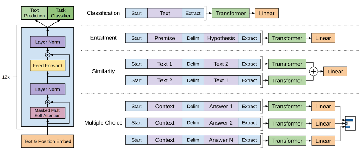
The genius of this work is how the authors structured the model input sequence so that it is possible to adapt the same model to a fairly diverse set of downstream tasks without changing the model architecture at all.
The following diagram explains this the best. The diagram shows that we would include a few special tokens: start, end ("Extract") and delimiter ("Delim"). The actually used tokens are <s>, <e>, \$. Here is a list of different tasks the model supports easily
- Classification: we only have one piece of input and attach the start and end tokens.
- Entailment is the classification of a text pair about their relationships. Here, we need the delimiter token to separate the premise and hypothesis text.
- Similarity: very similar to entailment, but since the task is symmetric, we'd predict both ordering [text1, text2] and [text2, text1], then sum their output element-wise, then feed that into the linear output layer.
- Multiple Choices: the context document $z$ and question $q$ are concatenated together first as the "Context" in the diagram. We then append a delimiter token and an answer $a_k$ (i.e., the input looks like $[z;q;\$;a_k]$ and do so over a set of possible answers $\set{a_k}$. Each of these sequences is processed independently with the model and then normalized via a softmax layer to produce an output distribution over possible answers.
During fine-tuning, we feed the sequence $x^1, ..., x^m$ (from labeled dataset $\mathcal C$ and properly structured with special tokens as discussed above) into the model and apply linear+softmax on top of the output $h_l^m$ of the last token at layer $l$ to predict the label $y$
$$p(y|x_1, ... x_m)= \mathrm{softmax}(h_l^m W_y)$$
This setup gives us the following objective to optimize over the dataset $\mathcal C$:
$$L_2(\mathcal C)=\sum_{(x,y)}{\mathrm {log}(p(y|x_1, ... x_m)} $$
The author proposed doing a weighted sum of the LM objective $L_1$ and the prediction objective $L_2$ when fine-tuning on dataset $\mathcal C$, thus the following is the objective:
$$L_3(\mathcal C) = L_1(\mathcal C) + \lambda L_2(\mathcal C)$$
The learnable parameter during fine-tuning is the weight in the final linear layer $W_y$ and the embedding of the special tokens.
2.3 BERT
BERT: Pre-training of Deep Bidirectional Transformers for Language Understanding (10/2018)
Overview
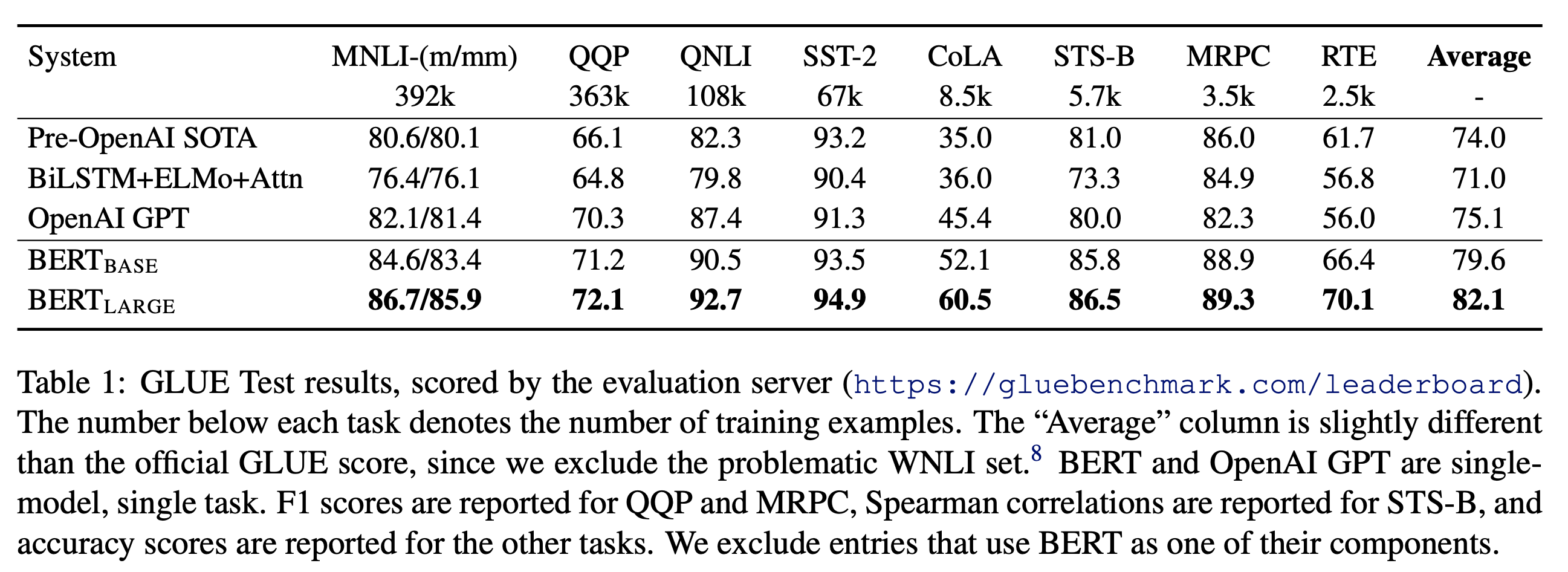
BERT came out within a few months of the GPT paper. I remember when it came out, it had more wow factor, perhaps due to its much stronger performance on downstream tasks - substantial improvements over GPT (see table below) as well as refreshed the record of multiple new tasks/leaderboard.
I think there isn't a lot of extra novelty in the BERT paper compared to that of GPT - as we will see the paper set up a slightly different way to use special tokens for downstream prediction tasks and used different pre-training objectives, but that's pretty much it. Nonetheless, strong performance is a strong performance. For a long period of time, BERT (and its variants) stayed at the top of the leaderboard and is all that people talk about, so the paper got a lot of citations, and the model is applied to many applications (e.g., semantic search, question answering, etc.).
I think the improved results are due to the following:
- A larger model (3X) and more training data (4X)
- Masked LM pre-training objective. Instead of only learning from preceding tokens (left context) in a conventional LM setup, the model can better represent the input and make predictions by considering both left and right context - making the model more data-efficient and with stronger prediction power.
- The next sentence prediction (NSP) pre-training objective complemented LM objective and led to strong model performance on tasks requiring understanding relationships between sentences, such as Q&A and NLI.
Model and pre-training data
The model the author used is the encoder part of the Transformer, with BERT-base having 100M parameters (i.e., similar to the GPT model) and BERT-large being 3X larger, having 340M parameters.
Recall that in the encoder of a Transformer, a few things differ from the decoder:
- The encoder model outputs a sequence of embeddings instead of predicting only the embedding for the next token. The length of this output sequence is the same as the input.
- At model input, it sees the entire sequence at once instead of future tokens being masked. (I think this is a contributor to BERT's better data efficiency, more on this later).
The model is pre-trained on both BooksCorpus (800M words, used in GPT paper) and English Wikipedia (2,500M words, with tables, titles, and lists ignored). Thus the training data size is 4X of the GPT paper. Similar to GPT, the author emphasized it is critical to use a document-level corpus rather than a shuffled sentence-level corpus such as the Billion Word Benchmark in order to extract long contiguous sequences.
Input/Output Representations
Let me cite the paper directly:
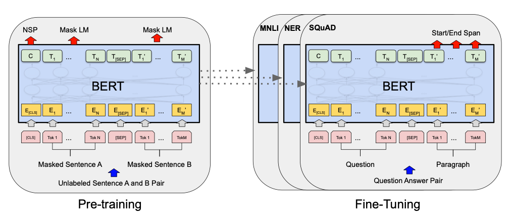
"The first token of every sequence is always a special classification token ([CLS]). The final hidden state corresponding to this token is used as the aggregate sequence representation for classification tasks. Sentence pairs are packed together into a single sequence. We differentiate the sentences in two ways. First, we separate them with a special token ([SEP]). Second, we add a learned embedding to every token indicating whether it belongs to sentence A or sentence B....we denote input embedding as E, the final hidden vector of the special [CLS] token as $C$, and the final hidden vector for the ith input token as $T_i$.
"For a given token, its input representation is constructed by summing the corresponding token, segment, and position embeddings."

Pre-training setup
Here is where BERT deviated from GPT substantially. The author did not use the transitional left-to-right language modeling (LM) objective, i.e., predicting the next token. Instead, they proposed two unsupervised tasks:
- Masked LM
- Next Sentence Prediction (NSP)
The Masked LM setup is interesting, where 15% of tokens in the input sequence is masked with a special token [Mask], and the final hidden vectors corresponding to the mask tokens are fed into an output softmax over the vocabulary, as in a standard LM - we test the model's ability to recover the masked word. This setup has been referred to as the Cloze task in some Q&A work.
The NSP task is geared to get the model ready for a few downstream tasks that involve understanding the relationship between two sentences, e.g., Question Answering (QA) and Natural Language Inference (NLI). This objective and capability aren't directly captured by language modeling. To construct the training example, we pick two sentences, and 50% of the time, swap the second sentence with a random sentence from the corpus. We use output C for prediction.
Adapting to downstream tasks
With similar special tokens, all the classification tasks we covered in GPT are straightforward to handle here as well - we can do linear+softmax over output $C$.
The paper also demonstrated BERT's performance on Q&A datasets such as SQuAD. In this, the context contains the answer, and the model is asked to predict the answer text span the context text. For this task, the author introduced a start vector $S \in \mathbb{R}^{d_{model}}$ and an end vector $E \in \mathbb{R}^{d_{model}}$ during fine-tuning. The probability of word $i$ being the start of the answer span is computed as a dot product between $T_i$ and $S$ followed by a softmax over all of the words in the paragraph. Same for the end. The training objective is the sum of the log-likelihoods of the correct start and end positions. At inference time, we can pick the span $[i,j]$ with the maximum score defined as $ST_i+ET_j$ .
2.4 GPT-2
GPT-2 Language Models are Unsupervised Multitask Learners (02/2019)
GPT-2 and GPT-3 are highly related, taking things in the same direction:
- Model size scaling (1000X between the first GPT paper and GPT-3)
- Zero-shot and few-shot learning (or "in-context" learning), no more updating pre-trained models
There are few differences in model architecture compared to the original GPT/Transformer block:
- GPT-2 vs GPT:
- LayerNorm is moved to the input of each Transformer block
- An additional layer normalization was added after the final selfattention block
- Modified initialization to account for deepr model
- GPT-3 vs GPT-2:
- Incorporating changes from Sparse Transformer
Language modeling = natural language prompt + multi-task learning
With the pre-training + fine-tuning setup (e.g., used in GPT and BERT), we still face the problem of needing a labeled dataset for each downstream task to do fine-tuning. This overhead limits model transferability to new tasks.
There was a fairly novel paper in 2018 from Salesforce Research: "The Natural Language Decathlon: Multitask Learning as Question Answering" (aka "DecaNLP"). In this work, the author cast a diverse set of tasks as question answering over a context and trained a single model to perform on all of them. Here the training is still supervised. Thus, we still need a labeled dataset for each task, and limitations of transferability to new tasks still apply. Below are some examples of this setting. Note that in this setup, the model is basically given a piece of text (Question+Context) and is asked to predict/generate another piece of text (Answer).
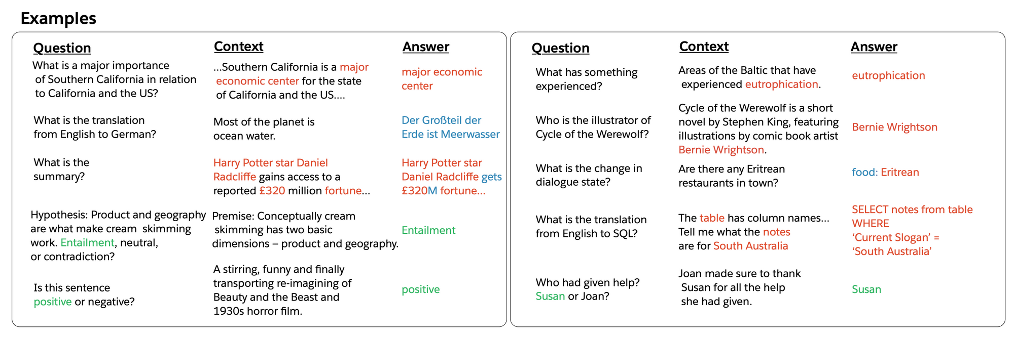
This setup looks remarkably suitable for language models - the supervised objective (multitask Q&A) is the same as the unsupervised objective (language modeling) but only evaluated on a subset of the sequence (the particular set of tasks), the global minimum of the unsupervised objective is also the global minimum of the supervised objective. GPT-2 draws inspiration from this work and continues the trend of more general methods of transfer. The key difference here is GPT-2 relies only on unsupervised learning (language modeling objective) and performs downstream tasks in a zero-shot setting – without any parameter or architecture modification.
To tell a pre-trained model what task to perform was previously achieved in GPT and BERT via a few special tokens (e.g., [CLS], [Extract/End]). However, in this zero-shot setting, we have no opportunity to fine-tune the model and let it know the meaning of these special tokens. Therefore, in GPT-2, the context and instructions for each task are completely represented by natural language - this is called "prompt" in later systems.
For example, a translation training example can be written as the sequence (translate to french, english text, french text). Likewise, a reading comprehension training example can be written as (answer the question, document, question, answer). "Translate to French" and "Answer the question" are the prompts in this case.
This zero-shot setting and using natural language prompts to guide a pre-trained language model to perform the downstream tasks is a daring step in GPT-2 (lots of credits also go to the DecaNLP paper mentioned earlier).
Model, data, and results
GPT-2 trained model similar to GPT paper but now with 1.5B parameters. The training data was created by scraping all outbound links from Reddit posts, which received at least 3 karma (a heuristic for the quality of the webpage). The resulting dataset is dubbed WebText, with 8 million documents for a total of 40 GB of text.

The zero-shot performance of GPT-2 is still far from the strong benchmarks of their task-specific and supervised learning counterparts. This is understandable - purely relying on a generic language modeling pre-training objective and not providing any task-specific supervision probably causes the model to be far less data-efficient compared to task-specific, supervised training.
Despite the current performance gaps, the trend of performance vs. model size scaling is very encouraging. Is there a ceiling? To test how far we can go, enter GPT-3.
2.5 GPT-3
GPT-3 Language Models are Few-Shot Learners (05/2020)
Overview
The key changes in GPT-3 are the following:
- 175B parameters, ~100X the model size compared to GPT-2
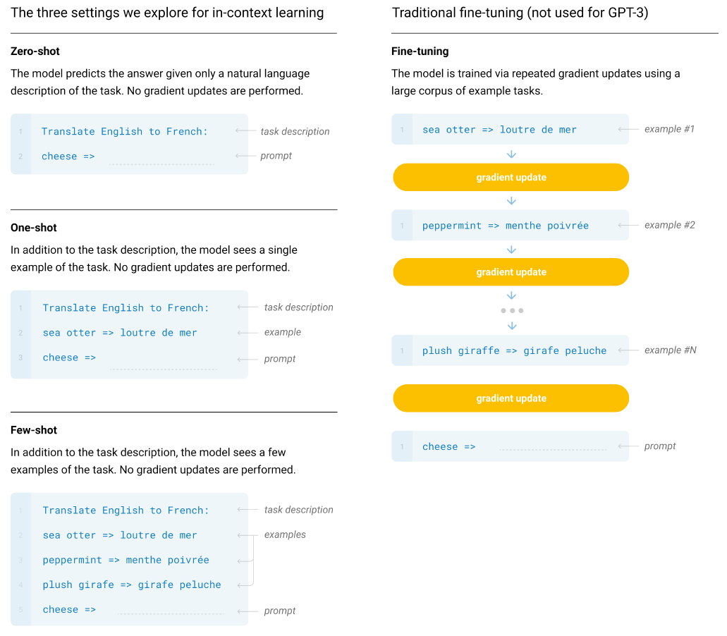
- Few-shot/"in-context" learning, i.e. provide models a few examples/demonstrations, still not updating model weights, but this is significant relaxation from zero-shot setting.
In order to train such a big model, the author assembled a dataset based on several sources with the most significant new addition of Common Crawl, details below:

The following figure illustrates the set of zero-shot, one-shot, and few-shot, contrasted with traditional fine-tuning. In the literature, few-shot learning often involves gradient updates to the model weight based on a few examples. Here the author used the term "in-context" learning to disambiguate with that and make it clear GPT-3 does not perform gradient updates in few-shot settings.
Results
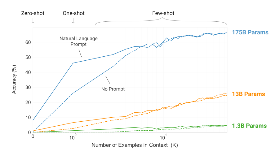
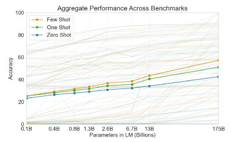
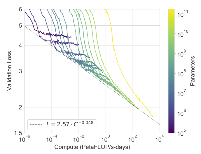
The GPT-3 technical report did extensive experiments. Here I want to cite a few graphs and briefly talk about the results qualitatively.
On benchmark datasets, GPT-3 consistently showed strong performance improvements over GPT-2. In some tasks, GPT-3's few-shot performance approaches or exceeds state-of-the-art (SOTA) results with task-specific models and/or fine-tuning. There are a couple of tasks GPT-3 seems to struggle with, more on that in the Limitations section later.
The clearest takeaways from the following several figures are:
- Few-shot massively improves performant over zero-shot (Figure 13)
- Power law scaling of performance vs model size (Figure 14) and compute increase (Figure 15), i.e. a linear performance increase requires an exponential increase in model size and compute.
These two explain massive improvements of GPT-3 over GPT-2 across tasks.
Limitations
First, the author pointed out the set of tasks GPT-3 struggles
- Text synthesis/generation: limited ability to generate long text with coherence, without repeating.
- Common sense physics/reasoning: e.g. “If I put cheese into the fridge, will it melt?”
- "Comparison" tasks, such as determining if two words are used the same way in a sentence or if one sentence implies another
The last category could be explained by the lack of bidirectional architecture (e.g. BERT) or denoising objective in GPT.
Beyond these more specific shortcomings, the author discussed a list of more general limitations. I found this section (Section 5 in the technical report) really insightful, summarized below:
- Limitations of LM objective: (1) indiscriminative learning of every token (2) forcing downstream tasks to be an LM compatible prediction problem rather than a more appropriate setup (3) lack of context beyond language (e.g. video, physical interactions)
- Poor pre-training data efficiency - broadly shared by language models.
- Large model, expensive, and inconvenient to perform inference.
- Unclear whether few-shot learning actually learns new tasks “from scratch” at inference time or if it simply recognizes and identifies tasks that it has learned during training. Though even the latter is already a major advance.
- Not interpretable.
In the report, there are also a lot of discussions about the broader impact to society, showing the team's thoughtfulness around it. I'd trust the mass media probably will spend the next several years talking about this so we can focus on the technical side of things in this note.
2.5 From GPT-3 to ChatGPT
From the official blog Introducing GhatGPT:
"We trained this model using Reinforcement Learning from Human Feedback (RLHF), using the same methods as InstructGPT, but with slight differences in the data collection setup. ... ChatGPT is fine-tuned from a model in the GPT-3.5 series, which finished training in early 2022."
Therefore, to create ChatGPT, the main ingredient apart from GPT-3 is InstructGPT, so in this section, we'll focus on it.
InstructGPT: Training language models to follow instructions with human feedback (3/2022)
Overview and key results
Fundamentally, GPT-3 is just a language model. When given a piece of text (i.e. prompt), it generates, somewhat randomly, plausible subsequent text that fits the best. This objective is misaligned with the goal of “following the user’s instructions helpfully and safely.” InstructGPT focuses on how to effectively align large language models such as GPT-3 with user intent through fine-tuning with human feedback so that the output can be more helpful, truthful and harmless.
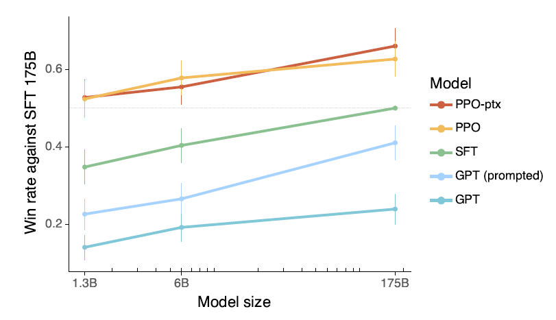
In human evaluations, outputs from the 1.3B parameter InstructGPT model are preferred to outputs from the 175B GPT-3, despite having 100x fewer parameters, demonstrating the effectiveness of the proposed alignment methods.
Alignment procedure
The figure below gives an excellent high-level overview of the procedure:
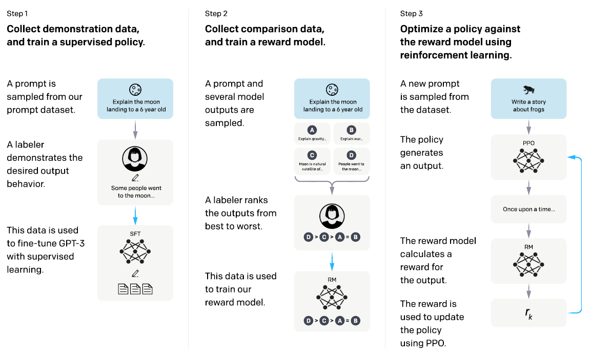
Step 1: Collect demonstration data, and train a supervised policy.
Here and below we can use the term "policy" and "model" interchangeably.
Step 1 is to fine-tune a pre-trained GPT-3 model on human-generated data. The model is called supervised fine-tuning (SFT). This SFT dataset is expensive to generate - it's largely based on labelers writing out actual questions and answers. This dataset has 13k prompts.
Step 2: Collect comparison data, and train a reward model.
Step 2 is to train a reward model (RM). The model predicts a single score for each pair of prompt and response. RM is a pseudo-labeler and a proxy of actual user feedback, so to speak. We will use its output as a cheap and efficient way to give SFT model feedback about whether the sampled output is good (i.e. truthful, helpful, harmless) during the reinforcement learning (RL) in Step 3.
RM model starts with SFT, removes the output linear+softmax layer at the output, and attaches a new linear layer to predict a scaler (instead of probability over vocabulary). The RM training data is a dataset of comparisons between model outputs, where labelers indicate which output they prefer for a given input. RM dataset has 33k training prompts.
RM is effectively a learning-to-rank model to correctly predict the rank order over $K$ responses using the following pairwise ranking loss:
$$\mathrm{loss}(\theta)=-\frac{1}{\binom{K}{2}}E_{(x, y_w, y_l)\sim D}[log(\sigma(r_\theta(x, y_w)-r_\theta(x, y_l)))]$$
where $r_\theta(x, y)$ is the scalar output of the reward model for prompt $x$ and completion $y$ with parameters $\theta$, $y_w$ is the preferred completion out of the pair of $y_w$ and $y_l$, and $D$ is the dataset of human comparisons.
Note that model inference cost scales linearly with $K$, but the number of pairwise training examples scale with $K^2$, while labeling cost scale sublinearly with $K$, thus making $K$ fairly large (e.g., 9 in the paper), is cost-effective.
Step 3: Optimize a policy against the reward model using PPO.
Now we have a fine-tuned model $\pi^{SFT}(y|x)$ and a reward model $r_\theta(x, y)$. We will use the reward model to find a more optimal parameter set $\phi$ for the model through a reinforcement learning (RL) set up:
- The environment is a bandit environment that presents a random customer prompt and expects a response to the prompt.
- Given the prompt and response, it produces a reward determined by the reward model and ends the episode.
We maximize the following combined objective function in RL training
$$\mathrm{objective}(\phi) = E_{(x,y)\sim \textcolor{orange}{D_{\pi_{\phi}^{RL}}}}\left[ \textcolor{red}{r_\theta(x,y)} - \textcolor{blue}{\beta \mathrm{log}\left(\frac {\pi_{\phi}^{RL}(y|x)}{\pi^{SFT}(y|x)}\right)}\right] + \textcolor{green}{\gamma E_{x \sim D_{pretrain}}\left[\mathrm{log}(\pi_{\phi}^{RL}(x)) \right]}$$
where $\pi_{\phi}^{RL}$ is the learned RL policy, $\pi^{SFT}$ is the supervised trained model, and $D_{pretrain}$ is the pretraining distribution.
The $\textcolor{red}{\mathrm{red}}$ portion of the objective is about maximizing reward. The $\textcolor{blue}{\mathrm{blue}}$ portion is the KL divergence between $\pi_{\phi}^{RL}$ and $\pi^{SFT}$, minimizing this KL term keeps the learned RL mode close to SFT and avoids overfitting of the reward model. The $\textcolor{green}{\mathrm{green}}$ portion is an added loss term to ensure the RL model keeps up its performance in the original language modeling objective - empirically, this helps $\pi_{\phi}^{RL}$ to continue perform well in common NLP tasks.
Note the first expectation term samples from the output generated by the RL model (the $\textcolor{orange}{\mathrm{orange}}$ part) rather than a static data distribution. This is why this is called RL, as the environment (where data is sampled from) is changing. This is also the reason PPO includes the KL term to limit over-optimization against reward and reward becoming inaccurate as $\pi_{\phi}^{RL}$ deviates too far from $\pi^{SFT}$ whose output samples trained the reward model.
Steps 2 and 3 can be iterated continuously; more comparison data is collected on the current best policy, which is used to train a new RM and then a new policy.
Conclusions & Reflections
ChatGPT really makes me feel excited about NLP and AI again. I'm in awe of the the progress made in the past five years.
Reflecting on the series of papers and milestones, here are a few thoughts and reactions, not particularly organized.
How much credit to give to Transformer?
Unsupervised learning really opened up more training data and model sizes for NLP. Looking back, I'm actually not sure how much of this scaling needs Transformer to happen. Can they still happen with just RNN/LSTM?
I haven't read the literature on the fundamental learning ability of Transformers. Did it break the bottleneck of the learning ability of CNN, RNN, and LSTM? Is that why we are able to keep scaling without saturating performance? This scaling is still expensive - power law of performance vs data/model, but having this brute force option is better than not having it.
Also, Transformers have fewer assumptions about the structure of the data. This nice property allows it to be applied to domains other than text, which helps those fields to scale as well.
Data Efficiency vs Performance Ceiling
BERT's performance beats GPT and GPT-2 at similar model sizes by a large margin. But later, GPT-3 based LM stunned the world, not BERT. Why?
BERT's setup to "fill in the blank" (Close style LM) is a simpler problem than left-to-right LM such as GPT. So, when the data and model are smaller, BERT's data efficiency gives it an edge on various performance benchmarks. Left-to-right LM is a more difficult and perhaps more generic task, allowing GPT with a sufficiently large training dataset to show strong performance eventually and, more importantly, the ability to generalize.
I'm really curious to see more results of very large (100B+ parameter models) with BERT-style bidirectional architecture and wonder whether it reaches similar or better performance than GPT but with much, much less data. Or do we see it plateau early?
Intelligence vs Memory
Looking at what ChatGPT can do, one might argue this is not really intelligence or reasoning: the model is hallucinating plausible answers based on its "memory" from pre-training without understanding what's going on. And, it can't explain how it came up with the answer even when the answers are correct and impressive.
That was my initial reaction too. But upon further thought, I think it is hard to disambiguate memory with intelligence, even for humans. Also, half of the time, we can't explain how we come up with something, either. So, I'd like to give a pass to the models on this one for now since we humans don't really understand what "understanding," "intelligence," and "ability to reason" are.
One thing we can still attack is that learning is relatively inefficient. GPT-3 kind of has exhausted the text from the Internet. Where do we go from here if we don't figure out how to be more sample efficient?
The future
We probably will see a flurry of activities of people using ChatGPT for all kinds of applications. We'll see everyone talking about this work and how it changes society forever. We'll see over-exaggerated expectations before more rational ones kick in - and generally, things probably follow the hype cycle thoroughly. I hope we can check our optimism and expectations sooner rather than later.
In the near term, GPT-3 and similar large language models (LLMs) will continue to be unruly - they are autoregressive in nature, they are prone to ramble off with plausible-sounding but bad answers and they are trained to do so. We won't really be able to directly and deterministically control its output to avoid toxicity, incorrect statements and flawed arguments.
To leverage their usefulness and avoid their baggage, we need new alignment methods (such as InstructGPT and more automated active learning with human feedback) and peripheral systems (such as information retrieval, moderation systems to reduce toxicity, fact-checking systems, etc.). While startups race to apply LLMs to various business verticals, I think formalizing and improving these peripheral systems as better control planes for LLMs is an important area ripe with opportunities.
Finally, for every field, there are a few core concepts. They're core, and for that reason, they are timeless and important to understand well. We are talking about things like entropy and other fundamental laws of physics and statistics. In the field of Artificial Intelligence, I hope we can continue to see steady progress in furthering the understanding of its core: the understanding of memory, intelligence, and the ability to reason.