Diffusion Models
This is the first post of hopefully a series of post walking through diffusion models. This post will introduce the foundations, focusing on two foundational papers, that many other papers built upon.

Overview
This is the first post of hopefully a series of post walking through diffusion models.
The slide version is at the bottom of this page.
This post will introduce the foundations, focusing on two foundational papers, that many other papers built upon.
Key papers
- [1a] Deep Unsupervised Learning using Nonequilibrium Thermodynamics (2015)
- Proposed the original Diffusion model for doing generative modelling.
- [1b] [DDPM] Denoising Diffusion Probabilistic Models (06/2020)
- Landmark paper, introduced a few key improvements (problem setup, model arch, loss function, etc), that are widely adopted by later papers.
Other resources
- This blog gives a good overview with approachable derivations What are Diffusion Models? | Lil'Log
- (I won’t repeat the derivations in this deck and instead focus on intuitions)
- 2022-08 Understanding Diffusion Models: A Unified Perspective
Generative Models
- What are generative models, when are they useful?
- Learns the data distribution and data generation process
- Useful anomaly detection (rare/no labels), compression, clustering (and other unsupervised learning problems).
- And of course, generating new data samples!
- Generate text, images, videos etc
- Learns the data distribution and data generation process
- Why is generative modeling hard?
- “Can you look at a painting and recognize it as being the Mona Lisa? You probably can. That's discriminative modeling. Can you paint the Mona Lisa yourself? You probably can't. That's generative modeling.” - Ian Goodfellow
- Deep generative models
- GAN
- Unstable adversarial training procedure. Lack of sample diversity.
- VAE
- Stable training. Lack of sample quality.
- Diffusion
- Stable training. Seems to do well in both quality and diversity.
- Note: Diffusion can be viewed as many (100~1000) VAEs chained together. Making the problem more incremental (more learnable?).
- GAN
Diffusion model, intuitions
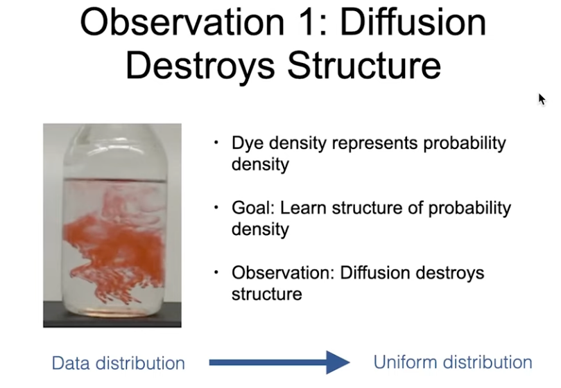
(source https://youtu.be/XCUlnHP1TNM?t=691)
- Observation 1:
- For generative models, often we need an “easy” distribution to begin with / sample from for generation and modeling of data distributions that are highly complex (e.g. real world images)
- Diffusion is a process that relates a complex distribution to a simple one.
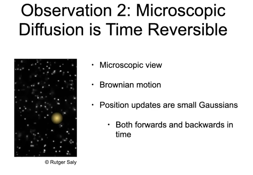
- Observation 2:
- At small time scale, diffusion is reversible, both the forward and reverse steps are Gaussian
- The ability to “learn” the (probabilistic) reversal step is due to the extra spatial information
- i.e. surrounding data points tell you what plausible arrangement could be in a previous time step


Diffusion model, formulation
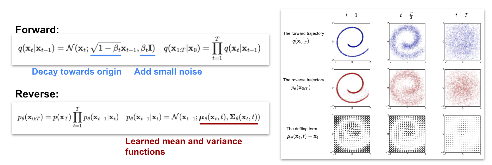
- We have a fixed forward diffusion process to convert data distribution to a known distribution (e.g. Gaussian)
- We have design choices about the forward process (e.g. what eventual distribution to converge to, how to evolve into it (noise schedule), etc).
- And a learned time reversal process to convert random samples from this known distribution (e.g. Gaussian) to a sample that follows data distribution (e.g. real image).
- We have design choices about how to parameterize the learned process/model (what model architecture, what optimization objectives, etc)

Learning objective
- The forward process q(xt | xt-1) is known, the reverse q(xt-1 | xt) is unknown. But…, if we know about the original image (x0), we can easily figure out the reverse trajectory q(xt-1 | xt, x0) (i.e. figure out how much noise is added to x0)
- Lots of algebra involved, but it is a simple Gaussian in the end.
- We do know about the original image x0 during forward process (we started from it), so we can q(xt-1 | xt, x0) as the ground truth to train a model pθ(xt-1 | xt) to guess/generate the reverse trajectory without knowing x0 beforehand.
- The learning objectively is: for all time step t, we’d like p to be very close to q
- We minimize the difference by minimizing KL divergence (usually denoted by DKL(q||p) it measures how different two distributions p and q are)
- So the learning objective below is a series of DKL terms covering all time steps t
- DKL between two Gaussian distributions has a simpler form: the difference between their means divided by covariance

Denoising Diffusion Probabilistic Models, aka DDPM
Landmark paper, made diffusion really work via a few key improvements that are widely adopted by later papers.
Key improvements details
- 1. predicting noise instead predicting image
- 2. Simpler loss objective, prioritized image generation quality instead of log likelihood
- 3. Better image model (U-Net with attention, more details in next slide)
DDPM, model details
- Used U-Net to model ptheta
- given a noised image, predict the noise, i.e. input and output both in the image dimensions
- Enhancements
- add self-attention (at 16x16 resolution between the convolution blocks)
- Diffusion time t is specified by adding Transformer sinusoidal position embedding into each residual block
- Code
(Ref: U-Net- Convolutional Networks for Biomedical Image Segmentation)
Side note: reconstruction error (distortion) vs time step
Going from t=T to t=0:
- We can stop at some t and try to directly take a guess of the original image (x0) and see how much we got wrong (“distortion”).
- We also count cumulatively from T to t, how much loss term Lt we accumulated (“rates”, infor theory parlance)

Takeaways
- The last few time steps (say t=0~10) accounts for large components in the overall loss. But they don’t contribute much to the improvements in reducing distortion of the reconstruction (image quality).
- This also calls to question whether we are wasting lots of model capacity on modeling details of the data distribution that are unimportant for generating realistic looking images (which is what motivated Latent Diffusion Model (LDM))

[Optional, but really interesting] Score-based models, unified with diffusion
Context
- Score-based models turned out to be equivalent to Diffusion (a somewhat accidental, concurrent development). It provides an alternative view of diffusion models.
- Score-based formulation helps derive very important methods for diffusion based image generation, e.g.
- Classifier- and Classifier-Free Guidance
- Accelerated sampling methods based on ODE solvers
- This section is not strictly needed for understanding most papers, read for curiosity but feel free to skip.
Key papers
- [1c] 2020-10 Generative Modeling by Estimating Gradients of the Data Distribution
- Will mostly focus on this one
- [1d] 2020-10 Improved Techniques for Training Score-Based Generative Models
- Various improvements over [1c]
- [1e] 2021-02 Score-Based Generative Modeling through Stochastic Differential Equations
- Casted the discrete time process into a continuous time domain and formulating it as an SDE (which helped later improvements on samplers based on numerical SDE/ODE solvers)
The author of these following papers wrote a phenomenal overview https://yang-song.net/blog/2021/score
See slides here for a summary https://docs.google.com/presentation/d/1CBthxtnEGbocgsferLSTCP6moQikm0id58EnOLPbfhk/edit#slide=id.g29442fbd5ed_0_416